Introduction
When it comes to finding the shortest path between two points in a graph, there are several algorithms available. Two of the most commonly used algorithms are Dijkstra's algorithm and Bellman-Ford algorithm. Both algorithms aim to find the shortest path in a graph, but they differ in their approach and application. In this article, we will explore the key differences between these two algorithms.
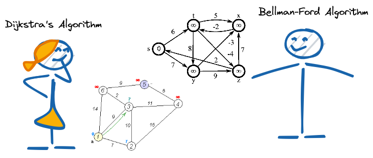
Dijkstra's algorithm is a greedy algorithm that starts at the source node and works its way outwards, exploring the graph in a breadth-first manner. It works by maintaining a set of unexplored nodes and a set of explored nodes. The algorithm picks the node with the shortest distance from the source node and adds it to the set of explored nodes. It then updates the distances of its neighbors if it finds a shorter path through the newly explored node. The algorithm continues this process until it has explored all nodes or until it reaches the destination node.
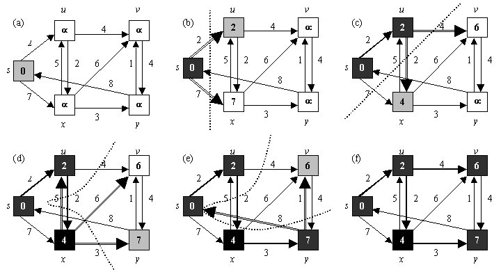
On the other hand, Bellman-Ford algorithm is a dynamic programming algorithm that works by relaxing the edges in the graph repeatedly. It starts by initializing the distance to the source node as 0 and the distance to all other nodes as infinity. It then iterates over all the edges in the graph, relaxing each edge and updating the distances of its endpoints. The algorithm repeats this process until it has relaxed all the edges in the graph or until it detects a negative cycle.
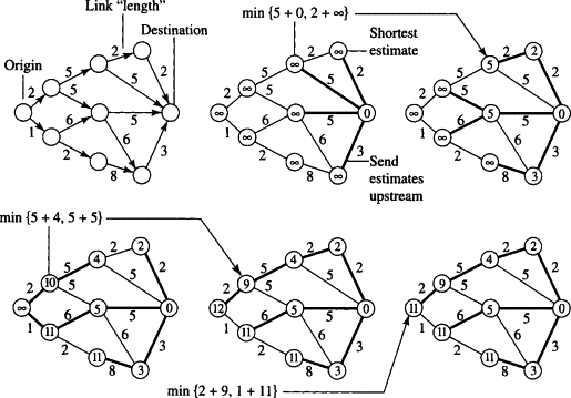
One of the key differences between Dijkstra's algorithm and Bellman-Ford algorithm is that Dijkstra's algorithm works only on graphs with non-negative edge weights, whereas Bellman-Ford algorithm works on graphs with negative edge weights as well. This is because Dijkstra's algorithm assumes that the shortest path to a node can be determined by examining its immediate neighbors, which is not always true in graphs with negative weights.
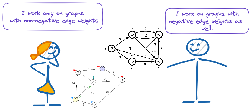
Another difference between the two algorithms is their time complexity. Dijkstra's algorithm has a time complexity of O(E log V), where E is the number of edges and V is the number of vertices in the graph. This is because it uses a priority queue to maintain the set of unexplored nodes, which has a logarithmic time complexity for insertion and removal. Bellman-Ford algorithm, on the other hand, has a time complexity of O(VE), where V and E are the number of vertices and edges in the graph, respectively. This is because it iterates over all the edges V-1 times to ensure that all the distances have been updated correctly.
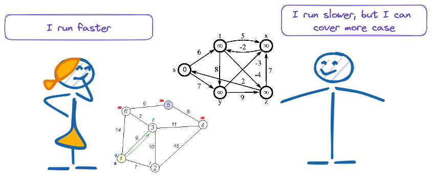
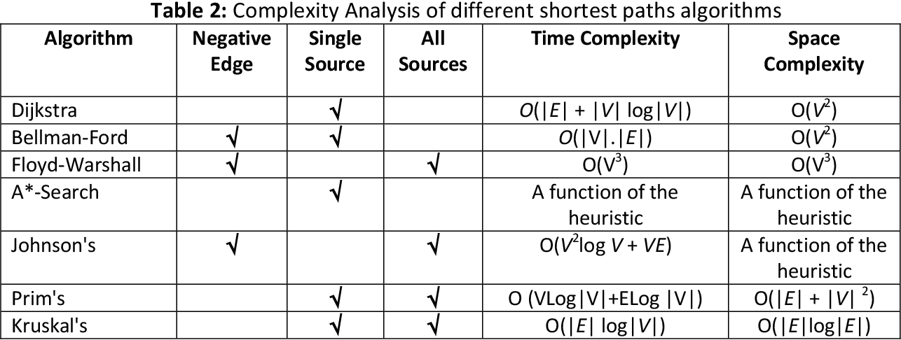
Let's see a table that summarizes the differences between Dijkstra's algorithm and Bellman-Ford algorithm about complexity :
A negative cycle in a graph is a cycle that has a negative weight. The presence of a negative cycle makes it impossible to determine the shortest path between two nodes in the graph. Both algorithms can detect negative cycles, but Dijkstra's algorithm assumes that there are no negative cycles in the graph and will fail if it encounters one. In contrast, Bellman-Ford algorithm can detect negative cycles and will return a message indicating that the graph contains a negative cycle.
Now, let's take a look at how these two algorithms work in practice.
Dijkstra's Algorithm
To demo Dijkstra's algorithm with the given data, we can follow these steps:
Step 1: Create the graph and initialize the algorithm
- Create an empty dictionary to represent the graph
- For each source, destination, and weight in the input, add an edge to the graph dictionary
- Initialize two dictionaries: 'distances' and 'visited'
- Set the distance of the startnode to 0 and the distances of all other nodes to infinity
- Set the startnode as the current node and mark it as visited
Here's the code for Step 1:
sources = [0, 0, 1, 1, 1, 2, 3, 3]
destinations = [1, 3, 2, 3, 4, 1, 2, 4]
weights = [6, 7, 5, 8, 1, 1, 1, 13, 9]
startnode = 0
endnode = 4
graph = {}

for i in range(len(sources)):
    source = sources[i]
    destination = destinations[i]
    weight = weights[i]
    if source not in graph:
        graph[source] = {}
    graph[source][destination] = weight
    if destination not in graph:
        graph[destination] = {}
    graph[destination][source] = weight

distances = {node: float('inf') for node in graph}
distances[startnode] = 0

visited = {}
current = startnode
visited[current] = TrueStep 2: Traverse the graph and update distances
- For each neighboring node of the current node, calculate the distance from the startnode to that node
- If the calculated distance is less than the current distance of the node, update the distance
- Mark the current node as visited and select the unvisited node with the smallest distance as the new current node
- Repeat until all nodes have been visited or the endnode has been reached
Here's the code for Step 2:
while current != endnode:
    for neighbor in graph[current]:
        distance = distances[current] + graph[current][neighbor]
        if distance < distances[neighbor]:
            distances[neighbor] = distance
    visited[current] = True
    unvisited = {node: distances[node] for node in graph if not visited.get(node)}
    if not unvisited:
        break
current = min(unvisited, key=unvisited.get)Step 3: Print the shortest path and distance to the endnode
If the endnode was not reached, print a message saying that there is no path Otherwise, print the shortest path and distance from the startnode to the endnode
Here's the code for Step 3:
if distances[endnode] == float('inf'):
    print("There is no path from", startnode, "to", endnode)
else:
    path = [endnode]
    while current != startnode:
        for neighbor in graph[current]:
            if distances[neighbor] == distances[current] - graph[current][neighbor]:
                path.append(neighbor)
                current = neighbor
                break
    path.reverse()
    print("Shortest path from", startnode, "to", endnode, "is", path)
print("Shortest distance is", distances[endnode])Result :
Shortest path from 0 to 4 is [0, 1, 4]
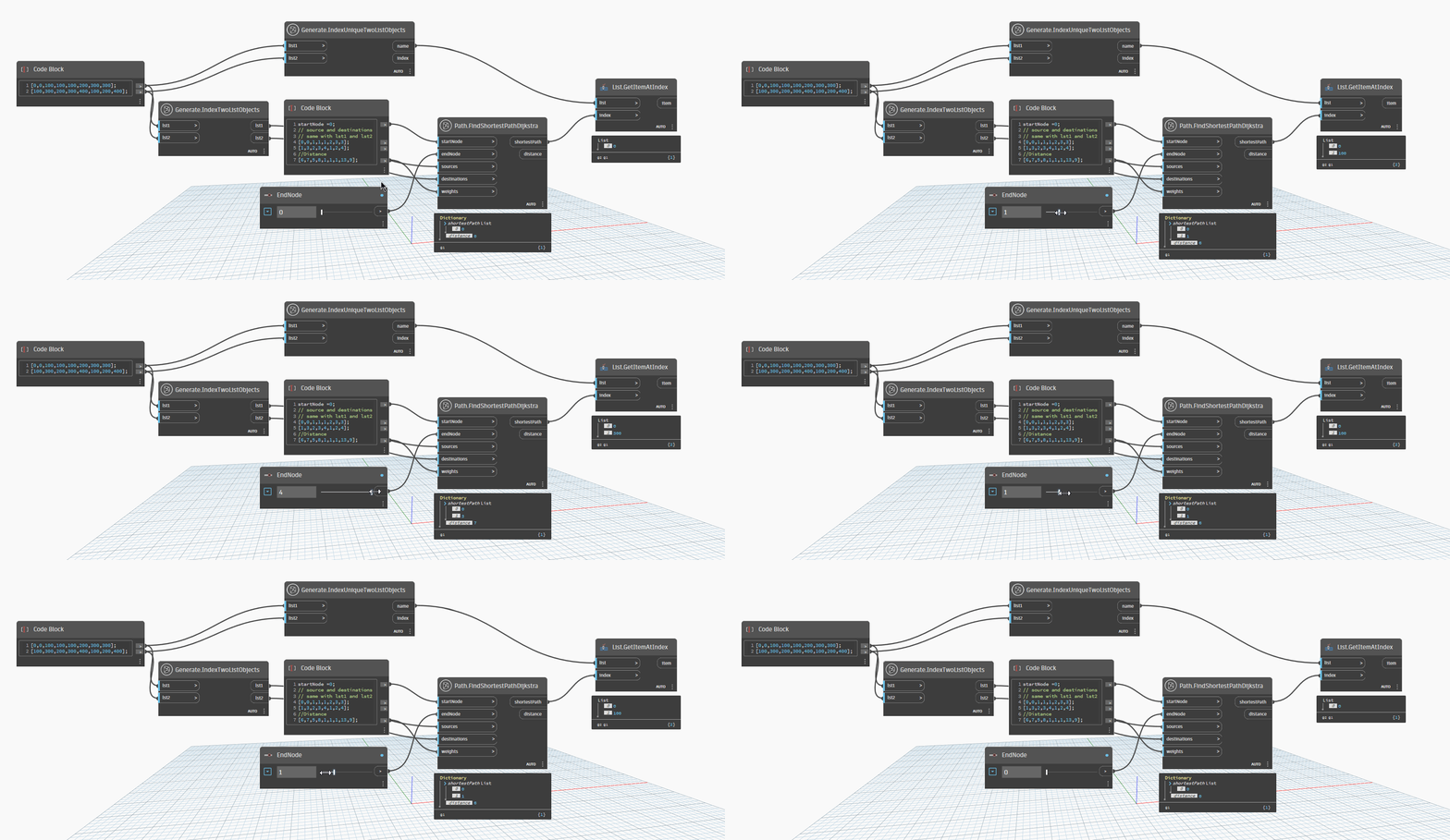
Shortest distance is 7Now, let's take a look at how the algorithm works in practice with Dynamo. In the image demo below, we try to find the shortest path from node 0 to node 4. Result is correct. with source input :
sources = [0, 0, 1, 1, 1, 2, 3, 3]
destinations = [1, 3, 2, 3, 4, 1, 2, 4]
weights = [6, 7, 5, 8, 1, 1, 1, 13, 9]
startnode = 0
endnode = 4Result also returns the output is the same with shortest path is [0,1,4] and shortest distance is 7. But we can use a input of endnode is slider to check other shortest path and shortest distance when endnode changed.
Bellman-Ford Algorithm
here's a step-by-step description of the Bellman-Ford algorithm:
Initialize the distances and predecessors for all nodes in the graph. Set the distance of the start node to 0 and the distance of all other nodes to infinity. Set the predecessor of all nodes to -1.
Relax the edges repeatedly for a maximum of N-1 times, where N is the number of nodes in the graph. To relax an edge, check if the sum of the distance of the source node and the weight of the edge is less than the distance of the destination node. If it is, update the distance of the destination node to be the sum of the distance of the source node and the weight of the edge, and update the predecessor of the destination node to be the source node.
Check for negative cycles by relaxing all the edges one more time. If any distance is updated during this step, then there is a negative cycle in the graph, and the algorithm cannot find the shortest path.
Build the shortest path by tracing the predecessors from the end node to the start node. Start at the end node and follow the predecessor links until you reach the start node. If there is no predecessor for a node, then there is no path from the start node to that node.
Return the shortest path and the distance of the end node from the start node.
this is the code for Bellman-Ford Algorithm :
def bellman_ford(sources, destinations, weights, startnode, endnode):
    # Step 1: Initialize distances and predecessors
    num_nodes = len(set(sources + destinations))
    distances = [float('inf')] * num_nodes
    distances[startnode] = 0
    predecessors = [-1] * num_nodes

    # Step 2: Relax edges repeatedly
    for i in range(num_nodes - 1):
        for j in range(len(sources)):
            source = sources[j]
            destination = destinations[j]
            weight = weights[j]
            if distances[source] + weight < distances[destination]:
                distances[destination] = distances[source] + weight
                predecessors[destination] = source

    # Step 3: Check for negative cycles
    for j in range(len(sources)):
        source = sources[j]
        destination = destinations[j]
        weight = weights[j]
        if distances[source] + weight < distances[destination]:
            return None

    # Step 4: Build the path
    path = [endnode]
    current = endnode
    while current != startnode:
        predecessor = predecessors[current]
        if predecessor == -1:
            return None
        path.append(predecessor)
        current = predecessor
    path.reverse()

return (path, distances[endnode])We can quick check result same with Dijkstra's algorithm.
sources = [0, 0, 1, 1, 1, 2, 3, 3]
destinations = [1, 3, 2, 3, 4, 1, 2, 4]
weights = [6, 7, 5, 8, 1, 1, 1, 13, 9]
startnode = 0
endnode = 4

result = bellman_ford(sources, destinations, weights, startnode, endnode)
if result is None:
    print("There is no path from", startnode, "to", endnode)
else:
    path, distance = result
    print("Shortest path from", startnode, "to", endnode, "is", path)
print("Shortest distance is", distance)Result :
Shortest path from 0 to 4 is [0, 1, 4]
Shortest distance is 7When the graph has negative cycles, the Bellman-Ford algorithm may not terminate, or it may return incorrect results.
This happens because the algorithm keeps relaxing the edges of the graph, which can cause the distance values to become smaller and smaller with each iteration. If there is a negative cycle in the graph, it means that there is a path that can be traversed indefinitely, causing the distance values to become infinitely negative.
The Bellman-Ford algorithm can detect negative cycles by performing one additional iteration of relaxation after N-1 iterations. If any distance value is updated during this additional iteration, then there is a negative cycle in the graph.
If the algorithm detects a negative cycle, it cannot find the shortest path because there is no shortest path in a graph with a negative cycle. In this case, the algorithm may return incorrect results, or it may not terminate at all.
Therefore, it is important to check for negative cycles before using the results of the Bellman-Ford algorithm. If a negative cycle is detected, the algorithm cannot be used to find the shortest path.
This is a code example to check negative cycle in the graph.
def has_negative_cycle(sources, destinations, weights, startnode):
    N = len(set(sources + destinations))
    distances = [float('inf') for i in range(N)]
    distances[startnode] = 0

    for i in range(N-1):
        for j in range(len(sources)):
            u, v, w = sources[j], destinations[j], weights[j]
            if distances[u] != float('inf') and distances[u] + w < distances[v]:
                distances[v] = distances[u] + w

    for j in range(len(sources)):
        u, v, w = sources[j], destinations[j], weights[j]
        if distances[u] != float('inf') and distances[u] + w < distances[v]:
            return True

    return False
result = has_negative_cycle(sources, destinations, weights, startnode)
print(result)Luckily, the result is False for example on top, so we can use Bellman-Ford Algorithm to find the shortest path for top example.
In image demo below, we try put some negative weights is -4, -2, -3 edges in the graph and use Bellman-Ford Algorithm to find the shortest path. Result is correct. this is one in advantage of Bellman-Ford Algorithm compare with Dijkstra's Algorithm. Let quick view image Visualizer in Dynamo Sandbox. We can change endnode one by one to see the shortest path from startnode to endnode.
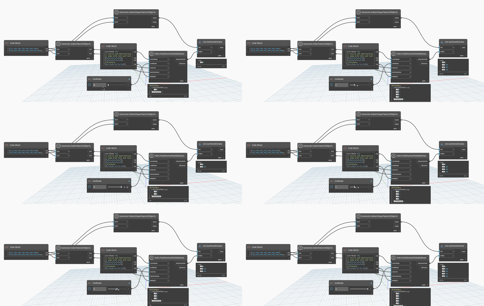
With Bellman-Ford algorithm, we can see the shortest path from startnode to all endnode and distance to endnode for each case, and the shortest path is result with distance smallest. This is a code example for that :
void Main()
{
	 BellmanFord bf = new BellmanFord(5, 8);
        bf.AddEdge(0, 1, 6);
        bf.AddEdge(0, 3, 7);
        bf.AddEdge(1, 2, 5);
        bf.AddEdge(1, 3, 8);
        bf.AddEdge(1, 4, -4);
        bf.AddEdge(2, 1, -2);
        bf.AddEdge(3, 2, -3);
        bf.AddEdge(3, 4, 9);

        Dictionary<int, Tuple<List<int>, int>> shortestPaths = bf.GetShortestPathsAndDistances(0);

        foreach (KeyValuePair<int, Tuple<List<int>, int>> entry in shortestPaths)
        {
            int vertex = entry.Key;
            List<int> path = entry.Value.Item1;
            int distance = entry.Value.Item2;

            Console.WriteLine("Shortest path from vertex 0 to vertex " + vertex + ": " + string.Join(" -> ", path));
            Console.WriteLine("Distance: " + distance);
            Console.WriteLine();
        }
}
public class BellmanFord
{
    private int V; // number of vertices
    private int E; // number of edges
    private List<Edge> edges; // list of edges
    private int[] distances; // array to store the distance from the source vertex to each vertex
    private int[] predecessors; // array to store the predecessor of each vertex in the shortest path

    public BellmanFord(int V, int E)
    {
        this.V = V;
        this.E = E;
        edges = new List<Edge>();
        distances = new int[V];
        predecessors = new int[V];
    }

    public void AddEdge(int src, int dest, int weight)
    {
        edges.Add(new Edge(src, dest, weight));
    }

    public void CalculateShortestPath(int src)
    {
        // initialize distances and predecessors
        for (int i = 0; i < V; i++)
        {
            distances[i] = int.MaxValue;
            predecessors[i] = -1;
        }
        distances[src] = 0;

        // relax edges V-1 times
        for (int i = 1; i < V; i++)
        {
            foreach (Edge edge in edges)
            {
                if (distances[edge.Src] != int.MaxValue && distances[edge.Src] + edge.Weight < distances[edge.Dest])
				{
					distances[edge.Dest] = distances[edge.Src] + edge.Weight;
					predecessors[edge.Dest] = edge.Src;
				}
			}
		}

		// check for negative-weight cycles
		foreach (Edge edge in edges)
		{
			if (distances[edge.Src] != int.MaxValue && distances[edge.Src] + edge.Weight < distances[edge.Dest])
			{
				throw new Exception("Graph contains negative-weight cycle");
			}
		}
	}

	public List<int> GetShortestPath(int dest)
	{
		List<int> path = new List<int>();
		int curr = dest;
		while (curr != -1)
		{
			path.Insert(0, curr);
			curr = predecessors[curr];
		}
		return path;
	}

	public int GetDistance(int dest)
	{
		return distances[dest];
	}

	public Dictionary<int, Tuple<List<int>, int>> GetShortestPathsAndDistances(int src)
	{
		// initialize dictionary
		Dictionary<int, Tuple<List<int>, int>> shortestPaths = new Dictionary<int, Tuple<List<int>, int>>();

		// calculate shortest path and distance for each vertex
		for (int i = 0; i < V; i++)
		{
			CalculateShortestPath(src);
			List<int> path = GetShortestPath(i);
			int distance = GetDistance(i);
			shortestPaths.Add(i, new Tuple<List<int>, int>(path, distance));
		}

		return shortestPaths;
	}

	private class Edge
	{
		public int Src { get; }
		public int Dest { get; }
		public int Weight { get; }

		public Edge(int src, int dest, int weight)
		{
			Src = src;
			Dest = dest;
			Weight = weight;
		}
	}
}Result :
Shortest path from vertex 0 to vertex 0: 0
Distance: 0

Shortest path from vertex 0 to vertex 1: 0 -> 3 -> 2 -> 1
Distance: 2

Shortest path from vertex 0 to vertex 2: 0 -> 3 -> 2
Distance: 4

Shortest path from vertex 0 to vertex 3: 0 -> 3
Distance: 7

Shortest path from vertex 0 to vertex 4: 0 -> 3 -> 2 -> 1 -> 4
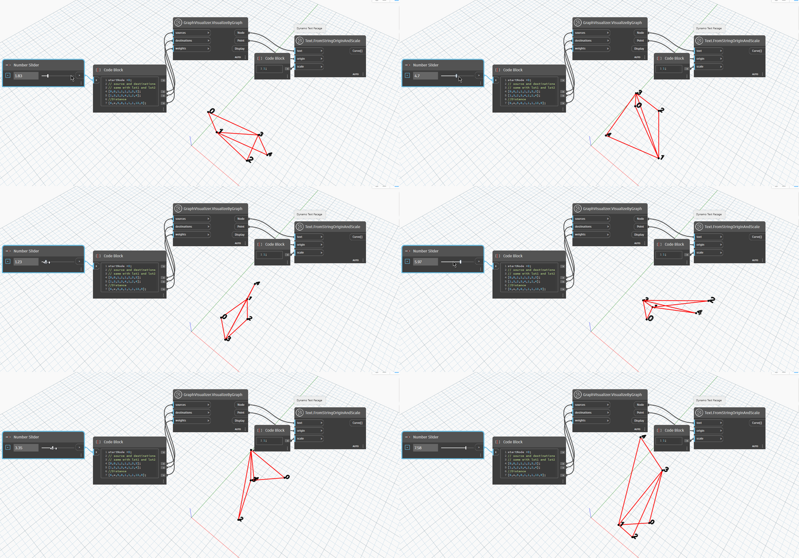
Distance: -2And I also created some node to visualize the shortest path in Dynamo Sandbox or Dynamo Revit. This is the code for VisualizeByGraph node with info, you can easily quick check for node 1 connect is : 0-1,1-2,1-3,1-4
 public static Dictionary<string,object> VisualizeByGraph(List<int> sources, List<int> destinations,
        List<double> weights)
    {
        // Create a dictionary to store the points for each vertex
        Dictionary<int, Vertex> points = new Dictionary<int, Vertex>();
        List<Modifiers.GeometryColor> display = new List<Modifiers.GeometryColor>();
        // Determine the maximum weight
        double maxWeight = double.MinValue;
        foreach (double weight in weights)
        {
            if (weight > maxWeight)
            {
                maxWeight = weight;
            }
        }

        // Create a 3D point for each vertex
        Random random = new Random();
        for (int i = 0; i < sources.Count; i++)
        {
            int source = sources[i];
            int destination = destinations[i];
            if (!points.ContainsKey(source))
            {
                Vertex vertex = new Vertex(Point.ByCoordinates(random.NextDouble() * maxWeight,
                    random.NextDouble() * maxWeight,
                    random.NextDouble() * maxWeight), source.ToString());
                points.Add(source, vertex);
            }

            if (!points.ContainsKey(destination))
            {
                Vertex vertex = new Vertex(Point.ByCoordinates(random.NextDouble() * maxWeight,
                    random.NextDouble() * maxWeight,
                    random.NextDouble() * maxWeight), destination.ToString());
                points.Add(destination, vertex);
            }
        }

        for (int i = 0; i < sources.Count; i++)
        {
            int source = sources[i];
            int destination = destinations[i];
            Vertex startVerText = points[source];
            Vertex endVerText = points[destination];
            display.Add(VisualizeByDestination(startVerText.Point, endVerText.Point));
        }
        return new Dictionary<string, object>()
        {
            {"Node", points.Values.Select(x=>x.Label).ToList()},
            {"Point", points.Values.Select(x=>x.Point).ToList()},
            {"Display", display}
        };
    }
Conclusion
In conclusion, Dijkstra's algorithm and Bellman-Ford algorithm are two widely used algorithms for finding the shortest path in a graph.
Dijkstra's algorithm is faster than Bellman-Ford algorithm for finding the shortest path in a graph with non-negative edge weights. This is because Dijkstra's algorithm visits each node only once and uses a priority queue to keep track of the smallest distance to each node. However, if the graph has negative edge weights, Dijkstra's algorithm may not work correctly, and Bellman-Ford algorithm should be used instead.
Bellman-Ford algorithm is slower than Dijkstra's algorithm in general, as it visits every node multiple times. However, it can handle graphs with negative edge weights and can detect negative cycles in the graph. Therefore, Bellman-Ford algorithm is useful when the graph has negative edge weights, or when we need to detect if there is a negative cycle in the graph.
In summary, Dijkstra's algorithm is a great choice when working with non-negative edge weight graphs and is generally faster than Bellman-Ford algorithm. However, if negative edge weights are present or negative cycles are suspected, Bellman-Ford algorithm is a better choice. Ultimately, the choice of algorithm depends on the characteristics of the graph and the problem at hand.
You can also try with other graph data to see the result with Dynamo by way download OpenMEP package and try explore with another practice.
